The Pseudopotential Method

The pseudopotential theory began as an extension of the OPW method. It is based on an ansatz which separates the total wave function into an oscillatory part and a smooth part, the so called pseudo wave function. The strong true potential of the ions is replaced by a weaker potential valid for the valence electrons.

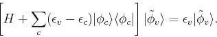
Philips and Kleinman (1959) showed that one can construct a smooth valence function $\tilde \phi_v$ that is orthogonal to the core states $\phi_c$, by using the following construction:

$$\vert\tilde \phi_v\rangle = \vert\phi_v\rangle + \sum_c \alpha_{cv}\vert\phi_c\rangle,$$ (219)

where the $\alpha_{cv}=\langle \phi_c\vert\tilde\phi_v\rangle$ are orthogonalization coefficients. This pseudo wave-function satisfies the modified Schrödinger equation:

$$\left[H+\sum_c(\epsilon_v - \epsilon_c)\vert\phi_c\rangle\la... ...rt\tilde \phi_v\rangle = \epsilon_v\vert\tilde \phi_v \rangle.$$ (220)

where $H = T+V$, and $V$ is the bare nuclear potential. This shows that it is possible to construct a pseudo-Hamiltonian

$$H_{PS} =H+\sum_c(\epsilon_v - \epsilon_c)\vert\phi_c\rangle\langle \phi_c\vert$$ (221)

with the same eigenvalues as the original Hamiltonian but smoother, nodeless wave function. The associated potential:

$$V_{PS} = V + \sum_c(\epsilon_v - \epsilon_c)\vert\phi_c\rangle\langle \phi_c\vert$$ (222)

was called a pseudopotential. This new correction is repulsive, and cancels the attractive potential enar the core, resulting into a smootha varying function.

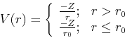
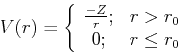
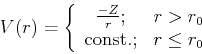
To simplify the problem even further, model pseudopotentials are used in place of the actual pseudopotential, for instace:

1. Constant effective potential in the core region
   

   $$V(r) = \left\{ \begin{array}{cc} \frac{-Z}{r}; & r > r_0 \\ \frac{-Z}{r_0}; & r \leq r_0 \end{array}\right.$$ (223)

   
   

2. Empty core model
   

   $$V(r) = \left\{ \begin{array}{cc} \frac{-Z}{r}; & r >r_0 \\ 0; & r \leq r_0 \end{array}\right.$$ (224)

   
   

3. model potential of Heine and Abarenkov:
   

   $$V(r) = \left\{ \begin{array}{cc} \frac{-Z}{r}; & r >r_0 \\ {\rm const.}; & r \leq r_0 \end{array}\right.$$ (225)

   
   

The solution of the problem is very simple. All these pseudopotentials have to be Fourier transformed to obtain the coefficients $V_{\bf K-K'}$, which are replaced in the OPW Schrödinger equation, which is in turn solved numerically.