


Next: The Ising model
Up: The Metropolis algorithm
Previous: The Metropolis algorithm
- simulate an ideal gas of
 particles in 1D. Choose
  ,
,  and 200 MC steps. Give all the particles the same initial velocity
 . Determine the value of the maximum velocity change
  so
that the acceptance ratio is approximately
so
that the acceptance ratio is approximately  . What is the mean
kinetic energy and mean velocity of the particles?
. What is the mean
kinetic energy and mean velocity of the particles?
- We might expect that the total energy of an ideal gas to remain
constant since the particles do not interact with each other and hence they
cannot exchange energy directly. What is the initial value of the energy
of the system? Does it remain constant? If it does not, explain how the
energy changes. Explain why the measured mean particle velocity is zero
even though the initial particle velocities are not zero.
- What is a simple criterion for ``thermal equilibrium''? Estimate the
number of Monte Carlo steps per particle necessary for the system to
reach thermal equilibrium. What choice of the initial velocities allows
the system to reach thermal equilibrium at temperature
 as quickly as
possible?
as quickly as
possible?
- Compute the mean energy per particle for
 ,
,  and
and  . In
order to compute the averages after the system has reached thermal
equilibrium, start measuring only after equilibrium has been achieved.
Increase the number of Monte Carlo steps until the desired averages do not
change appreciably. What is the approximate number of warmup steps for
. In
order to compute the averages after the system has reached thermal
equilibrium, start measuring only after equilibrium has been achieved.
Increase the number of Monte Carlo steps until the desired averages do not
change appreciably. What is the approximate number of warmup steps for
 and , and for
  and ? If the number of warmup
steps is different in the two cases, explain the reason for this
difference.
and ? If the number of warmup
steps is different in the two cases, explain the reason for this
difference.
- Compute the probability
 for the system of particles to
have a total energy between
for the system of particles to
have a total energy between  and
and  . Do you expect
  to be
proportional to
to be
proportional to  ? Plot as a function of and
describe the qualitative behavior of . Doe s the plot of
? Plot as a function of and
describe the qualitative behavior of . Doe s the plot of
 yield a straight line?
- Compute the mean energy for ,
 ,
,  ,
,  , and
, and
 and estimate the heat capacity.
- Compute the mean square energy fluctuations
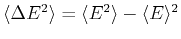 for and
 . Compare the magnitude of the ratio
 with the heat capacity determined in the previous item.
Next: The Ising model
Up: The Metropolis algorithm
Previous: The Metropolis algorithm
Adrian E. Feiguin
2009-11-04