Hydrogen atom

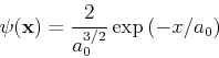
One example of the variational method would be using the Gaussian function $\chi(r) = e^{- \alpha r^2}$ as a trial function for the hydrogen atom ground state. This problem could be solved by the variational method by obtaining the energy of $\chi(r)$ as a function of the variational parameter $\alpha$, and then minimizing $E(\alpha)$ to find the optimum value $\alpha_{min}$. The variational theorem's approximate wavefunction and energy for the hydrogen atom would then be $\chi(r) = e^{- \alpha_{min} r^2}$ and $E(\alpha_{min})$.

This is a one electron problem, so we do not have to worry about electron-electron interactions, or antisymmetrization of the wave function. The Schrödinger's equation reads:

$$\left[ -\frac{\hbar^2}{2m}\nabla^2 - \frac{e^2}{4\pi\epsilon_0}\frac{1}{r} \right] \psi(x) = E \psi(x)$$ (36)

where the second term is the Coulomb interaction with the positive nucleus (remember, this is a charged particle in a central potential). The mass $m$ is the reduced mass of the proton-electron system, which is approximately equal to the electron mass. The ground state has energy

$$E=-\frac{N}{\hbar^2} \left(\frac {{\mathrm e}^2}{4\pi\epsilon_0} \right)^2 \approx -13.6058 {\mathrm eV}$$ (37)

and the wave function is given by

$$\psi({\bf x}) = \frac{2}{a_0^{3/2}} \exp{(-x/a_0)}$$ (38)

where $a_0$ is Bohr's radius

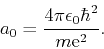$$a_0=\frac{4\pi\epsilon_0\hbar^2}{m{\mathrm e}^2}.$$ (39)

It is convenient to use units such that equations take on a simpler form. These are the so-called standard units in electronic structure: the unit of distance is Bohr's radius, masses are expressed in units of the electon mass $m_{\mathrm e}$, and charge in units of the electron charge e. The energy is finally given in ``hartrees'', equal to 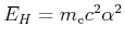$E_H=m_{\mathrm e}c^2\alpha^2$ (where $\alpha$ is the fine structure constant). In these units the Schrödinger equation for the hydrogen atom assumes the following simpler form:

$$\left[ -\frac{1}{2}\nabla^2 - \frac{1}{r} \right] \psi(x) = E \psi(x).$$ (40)

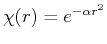
To approximate the ground state energy and wave function of the hydrogen atom in a linear variational procedure, we will use Gaussian basis functions. For the ground state, we only need angular momentum $l=0$ wave functions ($s$-orbitals), which have the form:

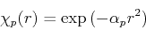$$\chi_p(r)=\exp{(-\alpha_p r^2)}$$ (41)

centered on the nucleus (whis is thus placed at the origin). We have to specify the values of the exponents $\alpha_p$, which are our variational parameters. Optimal values of these exponents have been previously found by other means, and in our case, we will keep these values fixed:

$$\alpha_1 = 13.00773$$ (42)

$$\alpha_2 = 1.962079$$ (43)

$$\alpha_3 = 0.444529$$ (44)

$$\alpha_4 = 0.1219492.$$ (45)

If the program works correctly, it should shield a value of the energy close to the exact results $E_0=-1/2 E_H$.

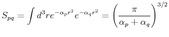
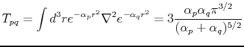
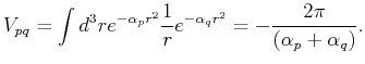
It remains to determine the coefficients of the linear expansion, by solving the generalized eigenvalue problem, as we did in the previous example. The matrix elements of the overlap matrix ${\bf S}$, the kinetic energy matrix ${\bf T}$, and the Coulomb interaction ${\bf V}$ are given by:

$$S_{pq} = \int d^3r e^{-\alpha_pr^2}e^{-\alpha_qr^2} = \left(\frac{\pi}{\alpha_p+\alpha_q}\right)^{3/2}$$ (46)

$$T_{pq} = \int d^3r e^{-\alpha_pr^2}\nabla^2 e^{-\alpha_qr^2} = 3 \frac{\alpha_p\alpha_q\pi^{3/2}}{(\alpha_p+\alpha_q)^{5/2}}$$ (47)

$$V_{pq} = \int d^3r e^{-\alpha_pr^2} \frac{1}{r} e^{-\alpha_qr^2} = - \frac{2\pi}{(\alpha_p+\alpha_q)}.$$ (48)

Using these expressions, one can fill the overlap and Hamiltonian matrices and solve the problem numerically.