The infinite potential well

The potential well with inifinite barriers is defined:

$$V(x) = \left\{ \begin{array}{ccc} \infty & {\mathrm for} &... ...thrm for} & \vert x\vert \leq \vert a\vert \end{array}\right.$$ (28)

and it forces the wave function to vanish at the boundaries of the well at $x=\pm a$. The exact solutioon for this problems is known and treated in introductory quantum mechanics courses. Here we discuss a linear variational approach to be compared with the exact solution. We take $a=1$ and use natural units such that $\hbar^2/2m=1$.

As basis functions we take simple polynomials that vanish on the boundaries of the well:

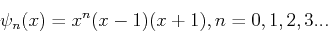$$\psi_n(x)=x^n(x-1)(x+1), n=0,1,2,3...$$ (29)

The reason for choosing this particular form of basis functions is that the relevant matrix elements can easily be calculated analytically. We start we the overlap matrix:

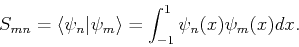$$S_{mn}=\langle \psi_n\vert\psi_m \rangle = \int_{-1}^1 \psi_n(x) \psi_m(x) dx.$$ (30)

Working out the integrals, one obtains

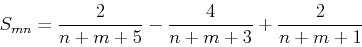$$S_{mn}=\frac{2}{n+m+5} - \frac{4}{n+m+3} + \frac{2}{n+m+1}$$ (31)

for $n+m$ even, and zero otherwise.

We can also calculate the Hamiltonian matrix elements:

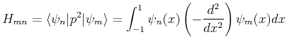$$H_{mn}=\langle \psi_n \vert p^2 \vert \psi_m \rangle = \int_{-1}^1 \psi_n(x) \left(-\frac{d^2}{dx^2} \right) \psi_m(x) dx$$ (32)

$$= -8 \left[ \frac{1-m-n-2mn}{(m+n+3)(m+n+1)(m+n-1)} \right]$$ (33)

for $m+n$ even, and zero otherwise.