Variational Methods

The variational method is an approximate method used in quantum mechanics. Compared to perturbation theory, the variational method can be more robust in situations where it is hard to determine a good unperturbed Hamiltonian (i.e., one which makes the perturbation small but is still solvable). On the other hand, in cases where there is a good unperturbed Hamiltonian, perturbation theory can be more efficient than the variational method.

The basic idea of the variational method is to guess a ``trial'' wavefunction for the problem, which consists of some adjustable parameters called ``variational parameters.'' These parameters are adjusted until the energy of the trial wavefunction is minimized. The resulting trial wavefunction and its corresponding energy are variational method approximations to the exact wavefunction and energy.

Why would it make sense that the best approximate trial wavefunction is the one with the lowest energy? This results from the Variational Theorem, which states that the energy of any trial wavefunction $E$ is always an upper bound to the exact ground state energy $E_0$. This can be proven easily. Let the trial wavefunction be denoted $\phi$. Any trial function can formally be expanded as a linear combination of the exact eigenfunctions $\psi_i$. Of course, in practice, we do not know the $\psi_i$, since we are assuming that we are applying the variational method to a problem we can not solve analytically. Nevertheless, that does not prevent us from using the exact eigenfunctions in our proof, since they certainly exist and form a complete set, even if we do not happen to know them:

$$\sum_{i,j}\langle\psi_{i}\vert\psi_{j}\rangle=\delta_{i,j}$$ (15)

where $\delta_{i,j}$ is the Kronecker delta.

$$H \left\vert\psi_i\right\rangle = E_i\left\vert\psi_i \right\rangle .$$ (16)

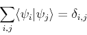
We are asuming that the physical states are normalized, i.e. their norm is equal to unity (we can always make it to do so). Let us assume that we have a candidate wavefunction to describe the ground-state, that we call $\vert\phi\rangle$, and that this function deppends on a set of parameters ${c_i}$, that we call variational parameters and are complex numbers. Ignoring complications involved with a continuous spectrum of H, suppose that the spectrum is bounded from below and that its greatest lower bound is $E_0$. So, the approximate energy corresponding to this wavefunction is the expectation value of $H$:

$$\left\langle\phi\vert H\vert\phi\right\rangle = \sum_{i,j} \left\langle\phi\vert\psi_{i}\right\rangle \left\langl... ...{i}\vert H\vert\psi_{j}\right\rangle \left\langle\psi_{j}\vert\phi\right\rangle$$ (17)

$$= \sum_{i} E_i \left\vert\left\langle\psi_i\vert\phi\right\rangle\r... ...\sum_{i}E_0 \left\vert\left\langle\psi_i\vert\phi\right\rangle\right\vert^2=E_0$$ (18)

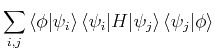
In other words, the energy of any approximate wavefunction is always greater than or equal to the exact ground state energy ${E}_0$. This explains the strategy of the variational method: since the energy of any approximate trial function is always above the true energy, then any variations in the trial function which lower its energy are necessarily making the approximate energy closer to the exact answer. (The trial wavefunction is also a better approximation to the true ground state wavefunction as the energy is lowered, although not necessarily in every possible sense unless the limit $\phi = \psi_0$ is reached).

Frequently, the trial function is written as a linear combination of basis functions, such as

$$\vert\phi\rangle = \sum_i c_i \vert\phi_i\rangle.$$

This leads to the linear variation method, and the variational parameters are the expansion coefficients $c_i$. We shall assume that the possible solutions are restricted to a subspace of the Hilbert space, and we shall seek the best possible solution in this subspace.

The energy for this approximate wavefunction is just

$$E[\phi] = \frac{\sum_{ij} c_i^* c_j \langle\phi_i \vert H\ver... ...angle}{ \sum_{ij} c_i^* c_j \langle\phi_i\vert\phi_j\rangle},$$ (19)

which can be simplified using the notation $H_{ij} = \langle \psi_i\vert H\vert\psi_j\rangle = \int \phi_i^* {H} \phi_j,$ $S_{ij} = \langle \psi_i\vert H\vert\psi_j\rangle = \int \phi_i^* \phi_j,$ to yield

$$E[\phi] = \frac{\sum_{ij} c_i^* c_j H_{ij}}{\sum_{ij} c_i^* c_j S_{ij}}.$$

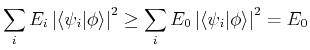
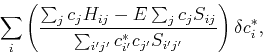
In order to find the optimial solution, we need to minimize this energy functional with respect to the variational parameters $c_i$, or calculate the variation such that:

$$\delta E({c_i})=0.$$ (20)

We will calculate only the variation with respect to $c_i^*$, since the variation with respect to $c_j$ will yield the same result:

$$\delta E = \sum_i \frac{\left(\sum_j c_j H_{ij} \sum_{i',j'} c_{i'}^*c_{j'} ... ...j'}\right)}{\left(\sum_{i',j'} c_{i'}^*c_{j'} S_{i'j'} \right)^2} \delta c_i^*.$$ (21)

Reordering some terms we can rewrite it as:

$$\sum_i \left(\frac{\sum_j c_j H_{ij} - E \sum_j c_j S_{ij}}{\sum_{i'j'} c_{i'}^*c_{j'} S_{i'j'}}\right) \delta c_i^*,$$ (22)

where $E$ is given by Eq.(19). This should be satisfied for all $c_i$'s, and we find that the coefficients should satisfy the following conditions:

$$\sum_{j=1}^N{(H_{ij}-ES_{ij})c_j} = 0 i=1,2,...,N.$$ (23)

This is a generalized eigenvalue problem, that can be rewritten:

$${\bf Hc}=E{\bf Sc},$$ (24)

where ${\bf H}$ is the Hamiltonian matrix, and ${\bf S}$ is the so-called ``overlap matrix''. The main difference with an ordinary eigenvalue problem is the marix ${\bf S}$ on the right hand side. We'll see how to solve this problem in the exercises. The solution to thsi problem is obtained by solving the following ``secular determinant''

$$\left \vert \begin{array}{cccc} H_{11} - E S_{11} & H_{12} ... ...2N} & \cdots & H_{NN} - E S_{NN} \end{array}\right\vert = 0.$$ (25)

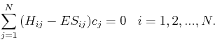
If an orthonormal basis is used, the secular equation is greatly simplified because $S_{ij} = \delta_{ij}$ (1 for $i=j$ and 0 for $i \neq j$), and we obtain:

$${\bf Hc}=E{\bf c},$$ (26)

which is nothing else but the stationary Schrödinger's equation, formulated in this basis. In this case, the secular determinant is

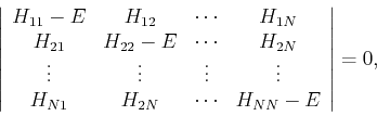$$\left \vert \begin{array}{cccc} H_{11} - E & H_{12} & \cdot... ...} & H_{2N} & \cdots & H_{NN} - E \end{array}\right\vert = 0,$$ (27)

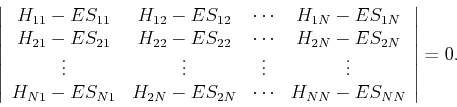
In either case, the secular determinant for $N$ basis functions gives an $N$-th order polynomial in $E$ which is solved for $N$ different roots, each of which approximates a different eigenvalue. These equations can be easily solved using readily available library routines, such as those in Numerical Recipes, or Lapack. At this point one may wonder where the approximation is: aren't we solving the problem exactly? If we take into account a complete basis set, the answer is ``yes, we are solving the problem exactly''. But as we said before, teh Hilbert space is very large, and we therefore have to limit the basis size to a number that is easily tractable with a computer. Therefore, we have to work in a constrained Hilbert space with a relatively small number of basis states kept, which makes the result variational. Because of the computer time needed for numerical diagonalizations scales as the third power of the linear matrix size, we would want to keep the basis size as small as possible. Therefore, the basis wavefunctions must be choses carefully: it should be possible to approximate the exact solution to the full problem with a small number of basis states. Inorder to do that, we need some good intuition about the underlying physics of the problem.

We have used a linear parametrization of the wave function. This greatly simplifies the calculations. However, nonlinear parametrizations are also possible, such as in the case of hartree-Fock theory.

The variational method lies behind hartree-Fock theory and the configuration interaction method for the electronic structure of atoms and molecules, as we will see in the following chapter.