We shall take a similar variational approach as the one used for the hydrogen atom. Let us take a wave-function of the form
 |
(71) |
![$\displaystyle \left[-\frac{1}{2}\nabla^2_{r_1} - \frac{Z}{r_1} + \sum_{r,s=1}^N...
...ac{1}{\vert{\bf r}_2-{\bf r}_2\vert} \right] \sum_{q=1}^N C_q \chi_q({\bf r}_1)$](img209.png) |
(72) | ||
 |
(73) |
 |
(74) |
 |
(75) | ||
 |
(76) | ||
| (77) |
Unfortunately, thsi is not a generalized eigenvalue equation because of the presence of the variables ![]() and
and ![]() inside the brackets on the left hand side. However, we can carry out a self-consistency iteration process as described earlier. By keeping
inside the brackets on the left hand side. However, we can carry out a self-consistency iteration process as described earlier. By keeping ![]() and
and ![]() fixed, we solve the equationo for the
fixed, we solve the equationo for the ![]() 's. We then replace the coefficients by the new solutiono, and iterate until convergence is achieved.
's. We then replace the coefficients by the new solutiono, and iterate until convergence is achieved.
In order to calculate the matrix elements, we shall use Gaussian ![]() basis functions, just as in the case of the hydrogen atom:
basis functions, just as in the case of the hydrogen atom:
| (78) |
| (79) | |||
| (80) | |||
| (81) | |||
| (82) |
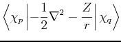
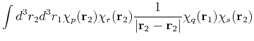
The matrix elements for the kinetic and Coulomb terms are similar to those calculated for the hydrogen atom, except for an extra factor of ![]() in the nuclear attraction. The matrix elements ofr
in the nuclear attraction. The matrix elements ofr ![]() are
are
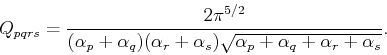 |
(83) |
The program is consructed as follows:
![]() First, the
First, the ![]() matrices
matrices ![]() ,
, ![]() and the
and the
![]() tensor
tensor ![]() are calculated.
are calculated.
![]() Initial values for the
Initial values for the ![]() coefficients are chosen (all equal, for instance).
coefficients are chosen (all equal, for instance).
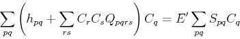
![]() These values are used to contruct the
These values are used to contruct the ![]() matrix given by
matrix given by
| (84) |
![]() We solve the generalized eigenvalue problem. For the ground-state, we keep only the eigenvector with the lowest eigenvalue.
We solve the generalized eigenvalue problem. For the ground-state, we keep only the eigenvector with the lowest eigenvalue.
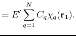
![]() We calculate the ground-state energy as:
We calculate the ground-state energy as:
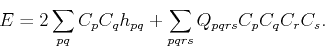 |
(85) |
![]() The new solution of the geenralized eigenvalue problem
is then used to contruct the new matrix
The new solution of the geenralized eigenvalue problem
is then used to contruct the new matrix ![]() and we repeat until the energy converges.
and we repeat until the energy converges.