Projector Monte Carlo

A simple modification of the Blankenbecler, Scalapino and Sugar algorithm allows the calculation of ground state properties in the canonical ensemble i.e. with a fixed number of electrons. This approach is called ``Projector Monte Carlo.'' Consider the ground state $\vert\psi _{0}\rangle$ of a system, and let us denote by $\vert\phi\rangle$ a trial state with a nonzero overlap with the actual ground state. If we apply the operator $P=e^{-\tau H}$a number $m$ of times over an arbitrary state $\vert\phi\rangle$, and we intercalate the identity operator in the basis $\vert\alpha\rangle$ of eigenstates of $H$, we obtain:

$$\vert\phi ^{m}\rangle = P^{m}\vert\phi \rangle$$

$$= \sum_{\alpha }e^{-m\tau H}\vert\alpha \rangle \langle \alpha \vert\phi \rangle$$

$$= \sum_{a}\left( e^{-\tau E_{\alpha }}\right) ^{m}\vert\alpha \rangle \langle \alpha \vert\phi \rangle$$

$$= e^{-\beta E_{0}}\sum_{a}\left( e^{-\tau (E_{\alpha }-E_{0})}\right) ^{m}\vert\alpha \rangle \langle \alpha \vert\phi \rangle .$$ (315)

In the limit with $\beta \rightarrow \infty$, the projection will filter out all the states with high energy and only the ground state will survive, i.e.

$$\lim_{m\rightarrow \infty }P^{m}\vert\phi \rangle =\mid \psi _{0}\rangle ,$$ (316)

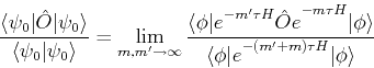
Thus, the ground state energy will be given by:

$$E_{0}={\frac{{\langle \phi \vert H\vert\psi _{0}\rangle }}{{... ...e }}{{\langle \phi \vert e}^{-m\tau H}{\vert\phi \rangle }% },$$ (317)

while for any othe physical observable ${\hat{O}}$, the expectation value can be exactly written as:

$${\frac{{\langle \psi _{0}\vert{\hat{O}}\vert\psi _{0}\rangle... ...e \phi \vert e}^{-(m^{\prime }+m)\tau H}{\vert\phi \rangle }}$$ (318)

This suggests that in principle, we can calculate the coeficients of the ground state of the system. However, we have to keep in mind that the dimension of the basis grows exponentially with the size of the lattice, and this will prevent us to keep in memory all the possible configurations. (Unless the system is small. Exercise for the reader: Heisenberg model on a chain with $N=4$ ).

The steps necessary to Monte Carlo simulate Eq.(321) are very similar to those discussed before in deriving Eq.(315). First, the imaginary time axis is discretized in a finite number of slices, then the Trotter approximation, as well as the Hubbard-Stratonovich decoupling are used. Fermions are integrated out, and all observables are finally expressed in terms of the spin-fields which are treated using a Metropolis algorithm (for details see Ref.[18]).

Another approach that uses the same principle consists in sampling the the ground state stochastically using a set of ''random walkers'' $\left\{ (w_{i},\vert x_{i}\rangle )\right\}$, where $w_{i}$ is a weight defined real and positive, and $\vert x_{i}\rangle$ are configurations usually in the $S^{z}$ or occupation number representations. The objective is to obtain a distribution of weights ans states that correspond to that of the actual ground state, generating a Markov chain applying stochastically the operator $P$

$$(w_{i}^{\prime },\vert x_{i}^{\prime }\rangle )\rightarrow P(w_{i},\vert x_{i}\rangle ).$$ (319)

The Projector Monte Carlo has been perfected over time, and the widely used scheme consists in using the projector operator:

$$G=[1-\tau (H-\omega )].$$ (320)

The quantity $\omega$ represents a good approximation of the ground state energy, and $\tau$ is a small time step that satisfies the condition $\tau \leq 2/(E_{\max }-\omega )$, where $E_{\max }$ is the maximum eigenvalue of $% H$. This variant is called Green Function Monte Carlo (GFMC). (See Refs. [4]-[7] and references therein)

In practice, several walkers are used simultaneously, with the first generation of walkers $\left\{ \vert x_{i}^{0}\rangle \right\}$ obtained using Variational Monte Carlo. This variational state is also used in the bias control and as guiding function for the importance sampling. The better the variational function, the lower the fluctuations in the mean values and the smaller the variance in the simulation. Both topics are out of the scope of this book, and the reader can find more information in the bibliography.