Next: World Line Monte Carlo
Up: Quantum Monte Carlo
Previous: Quantum Monte Carlo
We begin our description of the Quantum Monte Carlo variants with the
Variational Monte Carlo (VMC), the most transparent application of the ideas
described in previous sections. This algorithm is in the borderline that
divides the classical methods from the genuine quantum simulations.
Although quantum in nature, it is not the action of the
model that is sampled, but a trial wave function.
The main ingredient is a trial wave function
 , that depends on a set of parameters
 . This
wave function is represented in terms of a basis of orthogonal states
. This
wave function is represented in terms of a basis of orthogonal states 
where the coefficients of the parametrization are known functions of
 . We would like the wave function to be a good
representation of the actual ground state of a model. Finding the best wave
function means finding the right set of parameters
that
maximize the overlap with the actual ground state. In practice this is
impossible since we do not know the groud state a priori, and
some physical insight is needed to derive a good analytical
approximation. Then we apply the variational principle, that states
that the variational energy of the trial state is always greater or equal to
the exact energy of the ground state:
. We would like the wave function to be a good
representation of the actual ground state of a model. Finding the best wave
function means finding the right set of parameters
that
maximize the overlap with the actual ground state. In practice this is
impossible since we do not know the groud state a priori, and
some physical insight is needed to derive a good analytical
approximation. Then we apply the variational principle, that states
that the variational energy of the trial state is always greater or equal to
the exact energy of the ground state:
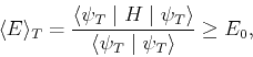 |
(278) |
and we use the criterium of minimizing the variational energy. In order to
do that we require to calculate this quantity for different sets of
parameters
, and once we found a proper wave function, we
can calculate the physical quantities of interest.
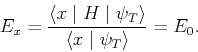
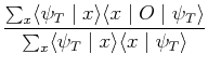
The expectation value of an arbitrary operator  is
is
with
 |
(281) |
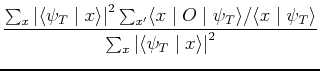
and
 |
(282) |
The equation (282) has precisely the form of a mean value in
statistical mechanics, with  as the Boltzmann factor:
The first step in order to calculate it consists of generating a collection
of configurations distributed according to this probability. For that
purpose we employ the Metropolis algorithm: starting from a configuration  , we accept a new configuration
 with
probability
with
probability
 , or
, or  if we
use the heat bath approach.
if we
use the heat bath approach.
The variational simulations are simple to perform and very stable.
Since the probabilities do not deppend on the statistics of the particles
involved, they do not suffer from the sign problem. However,
the results deppend decisively of the
quality of the variational wave function, because they are completely
pre-determined by it, and the physical arguments that define it. In the
particular situation in which the trial function coincides with the exact
ground state, the matrix elements (284) for  are all equal to
This is the property called ``zero variance'': the more the wave function
resembles the actual ground state, the more rapidly the variational enery
converges with the number of iterations.
In general, the computation results more complicated, or numerically more
expensive, when the number of variational parameters
that define the trial state is large. Thus, we always try to keep the form
of the wave function simple enough and with only a few variational degrees
of freedom.
Next: World Line Monte Carlo
Up: Quantum Monte Carlo
Previous: Quantum Monte Carlo
Adrian E. Feiguin
2009-11-04