Trajectories in phase space and integrability

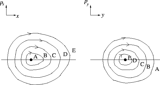
Figure 6: Trajectories of a particle in a two-dimensional separable potential as they appear in the $(x,p_x)$ and $(y,p_y)$ planes. Several trajectories corresponding to the same energy but different initial conditions are shown. Trajectories A and E area the limiting ones having vanishing $E_x$ and $E_y$, respectively

Let's ``complicate'' things a little bit. We know that all the problems described above can be expressed elegantly using the Hamiltonian formalism. Let us consider a particle of mass $m$ moving in a potential $V$ in two dimensions ans assume that $V$ is such that the particle remains confined if the energy is low enough. The momenta conjugate to the two coordinates $(x,y)$ area $(p_x,p_y)$. The Hamiltonian (the energy!) takes the form

$$H=\frac{1}{2}(p_x^2+p_y^2)+V(x,y).$$ (37)

Given any particular initial values of the coordinates and momenta, the particle's trajectory is specifies by their time evolution, that is governed by four first-order differential equations (Hamilton's equations):

$$\frac{dx}{dt}=\frac{\partial H}{\partial p_x}=p_x,\frac{dy}{dt}=\frac{\partial H}{\partial p_y}=p_y;$$ (38)

$$\frac{dp_x}{dt}=-\frac{\partial H}{\partial x} = -\frac{\partial ... ...frac{dp_y}{dt}=-\frac{\partial H}{\partial y} = -\frac{\partial V}{\partial y}.$$ (39)

For any $V$, these equations conserve the energy $E$ so that the constraint

$$H(x,y,p_x,p_y,t)=E$$

restricts the trajectory to a three-dimensional manifold embedded in the four dimensional phase space.

The Hamiltonian is said to be ``integrable'' when there is a second function of the coordinates and momenta that is also a constant of motion; the motion is thus constrained to a two-dimensional manifold in phase space. Two familiar kinds of integrable systems are separable and central potentials.

In the separable case

$$V(x,y)=V_x(x)+V_y(y)$$

where $V_{x,y}$ are independent functions of only one variable, so that the Hamiltonian separates in two parts and each coordinate can be solved independently,

$$H=H_x+H_y; H_{x,y}=\frac{1}{2}p_{x,y}^2+V_{x,y}.$$

The motions of $x$ and $y$ are therefore decoupled form each other and each of the Hamiltonians is separately a constant of motion.

In the case of a central potential,

$$V(x,y)=V(r); r=\sqrt{x^2+y^2},$$

so that the angular momentum $L_z=xp_y-yp_x$ is the second constant of motion and the Hamiltonian can be written as

$$H=\frac{1}{2}p_r^2+V(r)+\frac{p_{\theta}^2}{2r^2}.$$

where $p_r$ is the momentum conjugate to $r$. The additional constraint on the trajectory makes the system tractable reducing the problem to les variables. All the familiar analytically soluble problems in classical mechanics are those that are integrable. An analysis of phase space suggests a way to detect integrability. Consider for instance the case of a separable potential, Because the motions of each of the two coordinates are independent, plots of the trajectory in $(x,p_x)$ and $(y,p_y)$ planes should look as in Fig.6. Here, we assumed that each potential has a minimum value of 0 at particular values of $x$ and $y$ respectively. The particle moves on a closed contour in each of these two-dimensional projections of the four-dimensional phase space, each of them looking as a on-dimensional motion. The areas of these contours is associated to the total energy ($E_x$ and $E_y$). Since the total energy must be conserved, as one varies the initial conditions, one contour shrinks, and the other grows. In each plane there is a limiting contour that is approached when all the energy is in one coordinate. The fact that these contours are closed signals the integrability of the system.

How can we obtain this information from the trajectory alone? Supouse that at every time we observe one of the coordinates, say $x$, pass through zero, we plot the location of the particle in the $(y,p_y)$ plane. If the periods of the $x$ and $y$ motions are incommensurate (i.e. their ratio is an irrational number), then, as the trajectory proceeds, these observations will trace out the full $(y,p_y)$ contour; if the periods are commensurate (i.e. a rational ratio), then a series of discrete points around the contour will result.